Fast Robots - Lab 10: Localization [sim]

Overview

In this lab, we implemented grid-based localization using a Bayes Filter and simulated odometry. The goal was to estimate the position of a robot moving through a known map based on noisy sensor readings and control inputs. We executed this on a discretized grid using a virtual robot simulator.

The Bayes Filter

The Bayes Filter provides a probabilistic framework for estimating a robot’s position over time using control inputs (odometry) and observations (sensor measurements). Like the Kalman Filter, the Bayes Filter maintains a belief distribution over all possible positions and continuously refines it through prediction and update steps.

Algorithm Implementation

`compute_control()`

To model robot motion, we decomposed movement between two poses into:

A rotation toward the target position,
A translation to that location,
A final rotation to align with the desired orientation.

This function allows the filter to model motion in a structured, incremental way.

def compute_control(cur_pose, prev_pose):
    """ Given the current and previous odometry poses, this function extracts
    the control information based on the odometry motion model.

    Args:
        cur_pose  ([Pose]): Current Pose
        prev_pose ([Pose]): Previous Pose 

    Returns:
        [delta_rot_1]: Rotation 1  (degrees)
        [delta_trans]: Translation (meters)
        [delta_rot_2]: Rotation 2  (degrees)
    """
    x_cur = cur_pose[0]
    y_cur = cur_pose[1]
    ang_cur = cur_pose[2] * (math.pi / 180)

    x_prev = prev_pose[0]
    y_prev = prev_pose[1]
    ang_prev = prev_pose[2] * (math.pi / 180)
    
    r = math.sqrt((x_cur-x_prev)**2 + (y_cur-y_prev)**2)
    theta = math.atan2((x_cur-x_prev), (y_cur-y_prev))

    delta_rot_1 = (theta - ang_prev) * (180/math.pi)
    delta_trans = r
    delta_rot_2 = (ang_cur - ang_prev - delta_rot_1) * (180/math.pi)
    
    return delta_rot_1, delta_trans, delta_rot_2

`odom_motion_model()`

This function computes the probability of transitioning from prev_pose to cur_pose given a control input u, using Gaussian distributions around expected motion values.

Each sub-motion is assumed to be independent, and the product of their probabilities gives the total transition likelihood.

def odom_motion_model(cur_pose, prev_pose, u):
    """ Odometry Motion Model

    Args:
        cur_pose  ([Pose]): Current Pose
        prev_pose ([Pose]): Previous Pose
        (rot1, trans, rot2) (float, float, float): A tuple with control data in the format 
                                                   format (rot1, trans, rot2) with units (degrees, meters, degrees)

    Returns:
        prob [float]: Probability p(x'|x, u)
    """

    #odometry readings
    delta_rot_1, delta_trans, delta_rot_2 = compute_control(cur_pose, prev_pose)
    delta_rot_1 = mapper.normalize_angle(delta_rot_1)
    delta_rot_2 = mapper.normalize_angle(delta_rot_2)

    #ideal
    delta_rot_1_hat, delta_trans_hat, delta_rot_2_hat = u
    delta_rot_1_hat = mapper.normalize_angle(delta_rot_1_hat)
    delta_rot_2_hat = mapper.normalize_angle(delta_rot_2_hat)

    #compute probs
    p1 = loc.gaussian(delta_rot_1, delta_rot_1_hat, loc.odom_rot_sigma)
    p2 = loc.gaussian(delta_trans, delta_trans_hat, loc.odom_trans_sigma)
    p3 = loc.gaussian(delta_rot_2, delta_rot_2_hat, loc.odom_rot_sigma)

    prob = p1 * p2 * p3
    return prob

`prediction_step()`

We compute the prior belief bel_bar by looping through all potential past poses and computing the probability that the robot arrived at each new pose. For performance, we ignore states with negligible belief (e.g., < 0.0001).

This step models how motion spreads uncertainty in the belief space.

def prediction_step(cur_odom, prev_odom):
    """ Prediction step of the Bayes Filter.
    Update the probabilities in loc.bel_bar based on loc.bel from the previous time step and the odometry motion model.

    Args:
        cur_odom  ([Pose]): Current Pose
        prev_odom ([Pose]): Previous Pose
    """

    u = compute_control(cur_odom, prev_odom)

    cells_X, cells_Y, cells_A = mapper.MAX_CELLS_X, mapper.MAX_CELLS_Y, mapper.MAX_CELLS_A
    temp = np.zeros((cells_X, cells_Y, cells_A))

    for i in range(cells_X):
        for j in range(cells_Y):
            for k in range(cells_A):
                
                if(loc.bel[i,j,k] > .0001):
                
                    for a in range(cells_X):
                        for b in range(cells_Y):
                            for c in range(cells_A):

                                cur_pose = mapper.from_map(a,b,c)
                                prev_pose = mapper.from_map (i,j,k)
                                prob = odom_motion_model(cur_pose, prev_pose, u)
                                belief = loc.bel[i,j,k]
                                temp += prob * belief

    sum_val = np.sum(temp)
    loc.bel_bar = np.true_divide(temp, sum_val) ##normalized bel_bar

`sensor_model()`

The sensor model computes the likelihood of receiving the current sensor reading for each possible pose by comparing it to pre-cached ground truth sensor data.

def sensor_model(obs):
    """ This is the equivalent of p(z|x).

    Args:
        obs ([ndarray]): A 1D array consisting of the true observations for a specific robot pose in the map 

    Returns:
        [ndarray]: Returns a 1D array of size 18 (=loc.OBS_PER_CELL) with the likelihoods of each individual sensor measurement
    """
    prob_array = []
    
    for i in range(18):
        #create a gaussian distribuion for each meas
        gauss = loc.gaussian(loc.obs_range_data[i], obs[i], loc.sensor_sigma)
        prob_array.append(gauss)
    
    return prob_array

`update_step()`

In the update step, we combine the predicted belief with sensor likelihoods to compute a new, corrected belief distribution.

The final belief is normalized and used to localize the robot on the grid.

def update_step():
    """ Update step of the Bayes Filter.
    Update the probabilities in loc.bel based on loc.bel_bar and the sensor model.
    """

    cells_X, cells_Y, cells_A = mapper.MAX_CELLS_X, mapper.MAX_CELLS_Y, mapper.MAX_CELLS_A

    for i in range(cells_X):
        for j in range(cells_Y):
            for k in range(cells_A):
                p = sensor_model(mapper.get_views(i,j,k))
                prob = np.prod(p)
                loc.bel[i,j,k] = loc.bel_bar[i,j,k] * prob

    loc.bel = loc.bel / np.sum(loc.bel)

Simulation Results

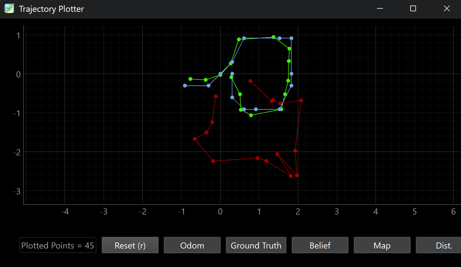
Our simulation showed that even with inaccurate odometry (red), the Bayes Filter (blue) was able to rapidly converge to the true position (green) of the robot. Despite large errors early in the trajectory, the filter corrected itself with sensor updates and achieved high accuracy.

Notably:

Errors were highest at corners of the grid but recovered quickly.
Raw Odom (red) is absolutely useless alone.
The center of the map occasionally produced ambiguous results
The belief consistently reached a confidence of prob = 1.0 at the correct grid cell.

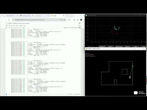
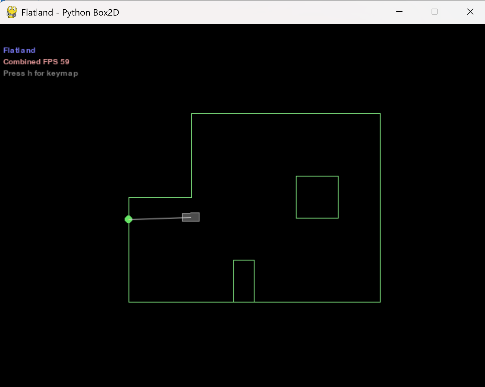
Localization Simulation

mapping

Discussion

The Bayes Filter proved highly effective for this task. Compared to the Kalman Filter, it supports non-linear motion and non-Gaussian distributions, making it more general and robust. It was particularly impressive how well the filter performed despite significant odometry drift.