
Fast Robots - Lab 11: Localization [real]
Bayes Filter [ simulation ]
In Lab 11, I implemented and tested grid-based localization on the real robot using a Bayes Filter. After verifying functionality in simulation, we deployed to hardware and collected real sensor data over BLE. The robot performed a full 360° rotation while logging yaw and distance (TOF) measurements, then used the Bayes Filter to infer its most probable location on a known map.
The simulation tests the Bayes Filter in a controlled environment. The red trajectory represents odometry-based motion prediction, the green line is ground truth, and the blue trajectory is the computed belief. The filter operates on a 3D grid (x, y, theta) and updates belief distributions at each step using odometry and sensor likelihood.
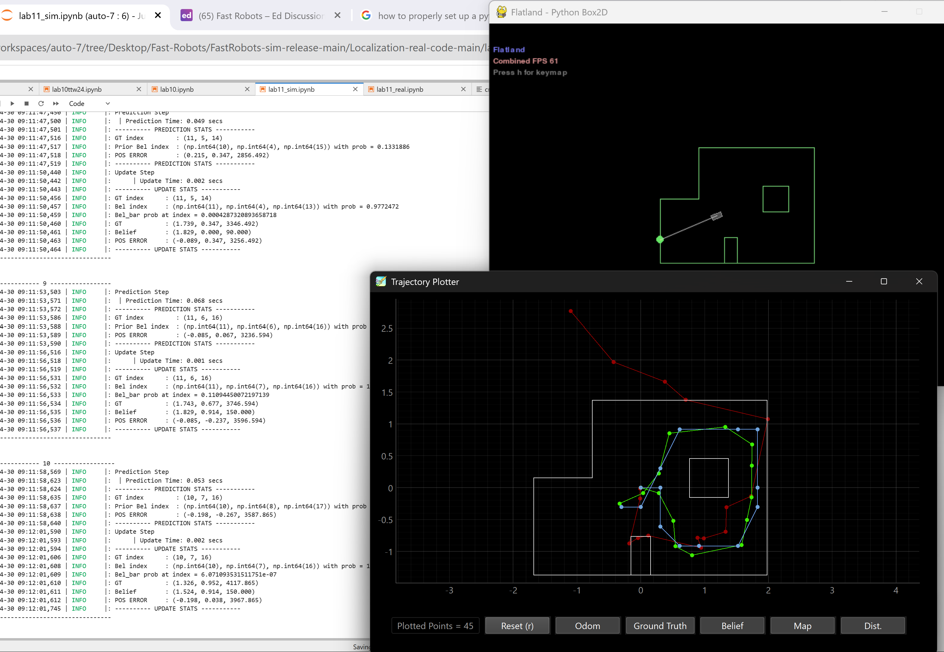
This part of the lab was unexpectedly time-consuming. I spent over 8 hours debugging environment mismatches, resolving dependency conflicts, and recreating virtual environments just to get the simulation running. Eventually, a clean reinstallation of Python and careful version management resolved the issues.
Bayes Filter [Real Robot]
The core functionality for the real robot was broken into two commands:
Artemis Code
This initiates the 360° rotation and sets up internal PID control for angular movement:
case ORIENTATION_CASE:
{
    success = robot_cmd.get_next_value(run_ORIENTATION_CASE);
    if (!success) return;
    success = robot_cmd.get_next_value(setAngle);
    if (!success) return;
    success = robot_cmd.get_next_value(Kp);
    if (!success) return;
    success = robot_cmd.get_next_value(Ki);
    if (!success) return;
    success = robot_cmd.get_next_value(Kd);
    if (!success) return;

    if (run_ORIENTATION_CASE == 1) {
        distanceSensor1.startRanging();
        delay(3000);

        // Reset state for collection
        yawV = PyawV = total = 0;
        count = end = 0;
        start = 1;
        b = i = h = 1;
        stop = 360 / setAngle;
        endTime = previousTime = millis();
    }

    Serial.print("run_ORIENTATION_CASE: ");
    Serial.print(run_ORIENTATION_CASE);
    Serial.print(" setAngle: ");
    Serial.print(setAngle, 4);
    Serial.print(" Kp: ");
    Serial.print(Kp);
    Serial.print(" Ki: ");
    Serial.print(Ki);
    Serial.print(" Kd: ");
    Serial.println(Kd);
}
break;
This command is used after the orientation routine completes, to send the yaw and distance data to the Python host:
case SEND_ORIENTATION_DATA:
{
    Serial.print("Sending orientation data...");
    for (int i = 0; i < 18; i++) {
        tx_estring_value.clear();
        tx_estring_value.append("T:");
        tx_estring_value.append(timePID_O[i]);
        tx_estring_value.append("|angle_arr:");
        tx_estring_value.append(yaw_arr[i]);
        tx_estring_value.append("|D1_mm:");
        tx_estring_value.append(distance_data[i]);
        tx_characteristic_string.writeValue(tx_estring_value.c_str());
    }
}
break;
Python Code
This Python function collects the data transmitted over BLE and parses it into yaw and distance readings:
import numpy as np
import asyncio

def perform_observation_loop(self, rot_vel=120):
    """
    Initiates a 360° rotation and collects 18 yaw/TOF readings from the real robot over BLE.
    """

    # Initialize observation arrays
    sensor_ranges = np.zeros((18, 1))
    sensor_bearings = np.zeros((18, 1))

    print("[INFO] Sending ORIENTATION_CASE command...")
    self.ble.send_command(CMD.ORIENTATION_CASE, f"1|{rot_vel}|1|0|0")  # run=1, setAngle=rot_vel, Kp=1, Ki=0, Kd=0

    print("[INFO] Waiting for motion to complete...")
    await asyncio.sleep(4.0)  # adjust depending on real spin time

    print("[INFO] Requesting data from robot...")
    self.ble.send_command(CMD.SEND_ORIENTATION_DATA, "")  # Triggers BLE data dump

    data_lines = []
    while len(data_lines) < 18:
        if self.ble.has_data():
            msg = self.ble.read_line().strip()
            if msg.startswith("T:"):
                data_lines.append(msg)
        else:
            await asyncio.sleep(0.01)

    print("[INFO] Parsing robot data...")
    for i, line in enumerate(data_lines):
        try:
            # Format: T:<time>|angle_arr:<yaw>|D1_mm:<distance>
            parts = line.split("|")
            yaw = float(parts[1].split(":")[1])
            dist_mm = float(parts[2].split(":")[1])
            dist_m = dist_mm / 1000.0

            sensor_ranges[i] = dist_m
            sensor_bearings[i] = yaw
        except Exception as e:
            print(f"[WARN] Skipped malformed line: {line}, Error: {e}")

    self.obs_range_data = sensor_ranges
    return sensor_ranges, sensor_bearings
The belief distribution is compared to the known ground truth location of the robot. The Bayes Filter output is visualized using cmdr.plot_gt() to mark true poses and compare them against the computed belief.
# cmdr.plot_gt(-0.9144,-0.6096) # -3,-2 = -0.9144, -0.6096
# cmdr.plot_gt(1.524,0.9914) # 5, 3 = 1.524, 0.9144
# cmdr.plot_gt(1.524,-0.9914) # 5, -3 = 1.524, -0.9144
cmdr.plot_gt(0,0.9914) # 0, 3 = 0, 0.9144
After testing, I plotted ground truth vs computed belief. Ground truth is green and comupted is blue.
(-3,-2)
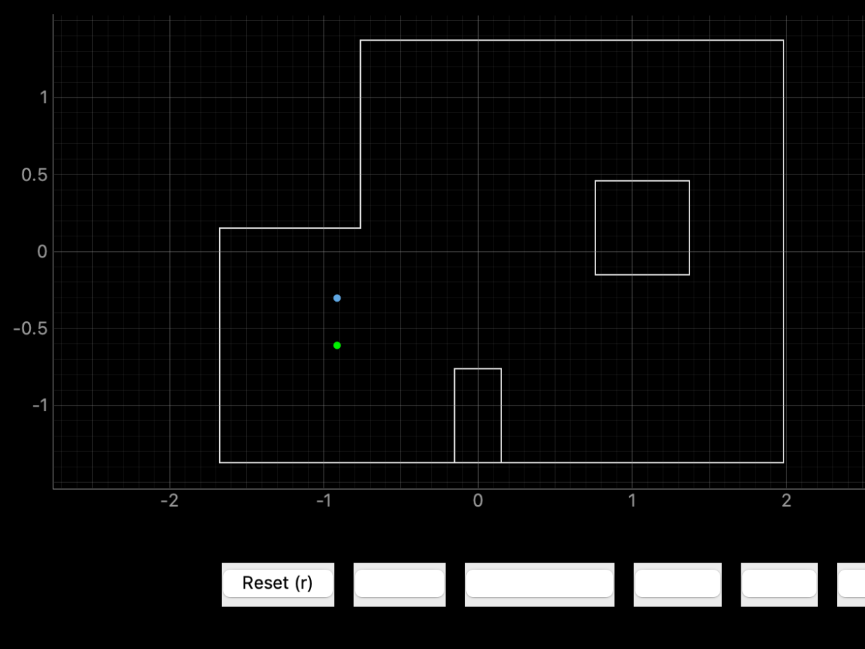
Ground truth pose: (-0.914, -0.914, 0.000)
Computed belief pose: (-0.914, -0.304, 60.0)
Resultant error: (0.000, 0.610, 60.0)
(5,3)
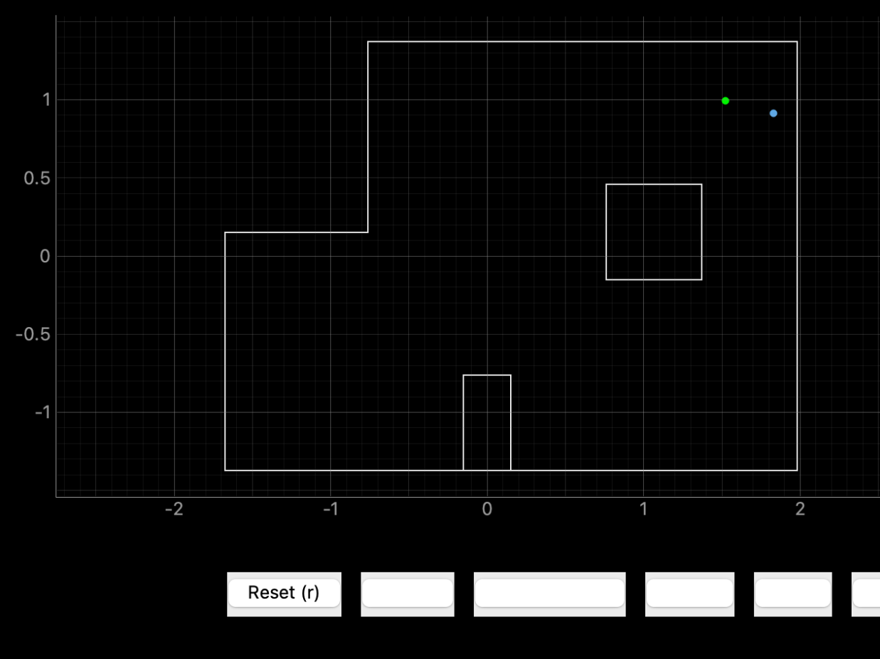
Ground truth pose: (1.524, 0.914, 0.000)
Computed belief pose: (1.821, 0.852, 70.0)
Resultant error: (0.297, 0.062, 70.0)
(5,-3)
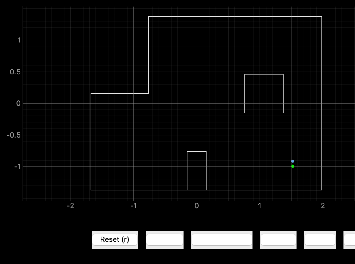
Ground truth pose: (1.524, -0.914, 0.000)
Computed belief pose: (1.524, -1.054, 10.0)
Resultant error: (0.000, 0.140, 10.0 )
(0,3)
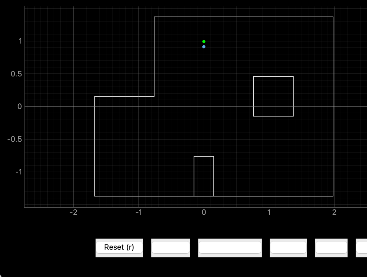
Ground truth pose: (0.000, 0.914, 0.000)
Computed belief pose: (0.000, 0.904, -10.0)
Resultant error: (0.000, 0.010, 10.0)
Conclusion
While not perfect, the Bayes Filter performed well under real-world noise. The largest errors occurred in orientation rather than position, which is expected given the limitations of single-sensor range-only localization with a fairly large (20 degree) swing between measurements. While not perfect, the Bayes Filter performed well under real-world noise. The largest errors occurred in orientation rather than position, which is expected given the limitations of single-sensor range-only localization with a fairly large (20 degree) swing between measurements.