Fast Robots - Lab 5: Linear PID

Prelab

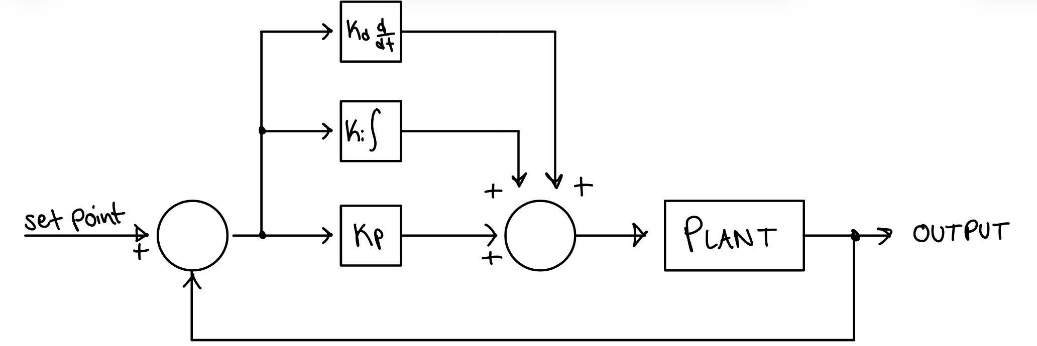
The purpose of this lab was to implement closed loop control through PID controllers. The state I controlled was speed, and I used the TOF sensors to stop a set distance from the wall. PID stands for proportional, integral, derivative control.

Bluetooth Communication Setup

For this lab, I implemented a robust Bluetooth communication system to send and receive data between the Artemis and my computer. This was essential for debugging and tuning the PID controller. I tried to use a flag-based system to start and stop the PID control loop remotely, but kept encountering errors or inconsistency. Instead I ended up adding a Stop PID function which would cut power to the motors. In practice, I didn’t end up using this at all though and just unplugged the power.

case START_PID:
{
    // to fill in later
}

case STOP_PID:
{
  PID_ON = false;
            
            pinMode(motor1a, OUTPUT);
            pinMode(motor1b, OUTPUT);

            pinMode(motor2a, OUTPUT);
            pinMode(motor2b, OUTPUT);

            analogWrite(motor1a,0);
            analogWrite(motor1b,0);

            analogWrite(motor2a,0);
            analogWrite(motor2b,0);
}

Figure 1: PID BLE control

Additionally, I implemented a helper function for driving in a straight line. I also added a stop driving variation if I set dir=0 or at least not +/-1:

void driveStraight(int dir, int PWM){
  if (dir == 1){
    //drive forward
    analogWrite(motor1a, 0);
    analogWrite(motor1b, int(PWM*cal));
    analogWrite(motor2a, PWM);
    analogWrite(motor2b, 0);
  }
  else if (dir == -1){
    //drive backward
    analogWrite(motor1a, int(PWM*cal));
    analogWrite(motor1b, 0);
    analogWrite(motor2a, 0);
    analogWrite(motor2b, PWM);
  }
  else {
    analogWrite(motor1a, 0);
    analogWrite(motor1b, 0);
    analogWrite(motor2a, 0);
    analogWrite(motor2b, 0);
  }
}

Figure 2: Bluetooth command to update PID gains

Lab Tasks

P/I/D Discussion

I started with a Proportional (P) controller to control the robot’s speed and position relative to the wall. The P controller calculates the error as the difference between the target distance (305 mm) and the current distance measured by the ToF sensor. The PWM output is proportional to this error.

I had a ton of trouble with this part of the lab. Many errors and code rewrites, memory issues, and I even reworked my mounting structure for my ToF sensors. After much simplification, I was able to achieve a pretty effective P control setup using the following code.

case PID_BEGIN:{

    int count = 0;
    int distance = 0;
    int pwm=0;
    int dir= 1;
    int err=0;

    while (currMillisTOF - prevMillisTOF <= 10000) {
        distanceSensor1.startRanging();

        if (distanceSensor1.checkForDataReady()) {
        time_array[count] = (int)millis();

        //Serial.print("tof: ");
        distance = distanceSensor1.getDistance();
        distanceSensor1.clearInterrupt();
        distanceSensor1.stopRanging();
        //Serial.print(distance);
        TOF_array[count] = distance;

        err = (int)(distance - targetDist );
        pwm= (int) (kp*err);

        //Serial.print("    dir: ");

        if (err > 0){
            dir=1;
            //Serial.print(" forward    ");

        }

        else if (err < 0){
            dir= -1;
            //Serial.print(" backward    ");
        }
        pwm= abs(pwm);

        if (pwm < pwmMin ) pwm = pwmMin;
        if (pwm > pwmMax ) pwm = pwmMax;

        //Serial.println(pwm);

        driveStraight(dir, pwm);
        PWM_array[count] = (dir*pwm);
        //currMillisTOF = millis();
        count++;
        }
    }

    driveStraight(0, 0); //stop driving

    for (int i = 0; i < count; i++) {
        tx_estring_value.clear();
        tx_estring_value.append(time_array[i]);
        tx_estring_value.append(" | ");
        tx_estring_value.append(TOF_array[i]);
        tx_estring_value.append(" | ");
        tx_estring_value.append(PWM_array[i]);
        tx_characteristic_string.writeValue(tx_estring_value.c_str());
    }
        delay(10000);
        driveStraight(-1, 100);
        delay(1000);
        driveStraight(0, 0); //stop driving
        delay(10000);
}

Figure 3: Proportional control implementation

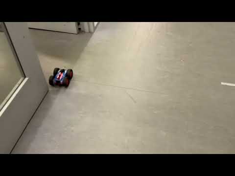
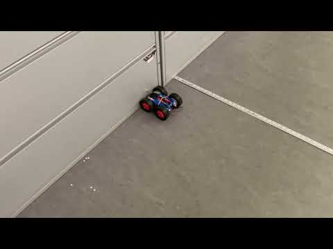
After tuning, I found that a Kp value of 0.07-5 worked well for me. Higher values caused signifigant overshoot where the robot would sometimes hit the wall. As such I added a bolt to front of my car so I don’t damage the ToF sensor. I also added a line to drive my car back to me after I was done.

I also added a lengthy delay to the end so I can pick up and turn off my car. For some reason, my car would automatically start running random case statements after I was already done. I never called them myself. I don’t know why this is happening and I haven’t found a solution, but it’s not that disruptive so I’ve just decided to live with it for now. I hope I can figure it out in lab.

Big Kp

Overshoot with Kp=0.07

Pretty good with Kp=0.05

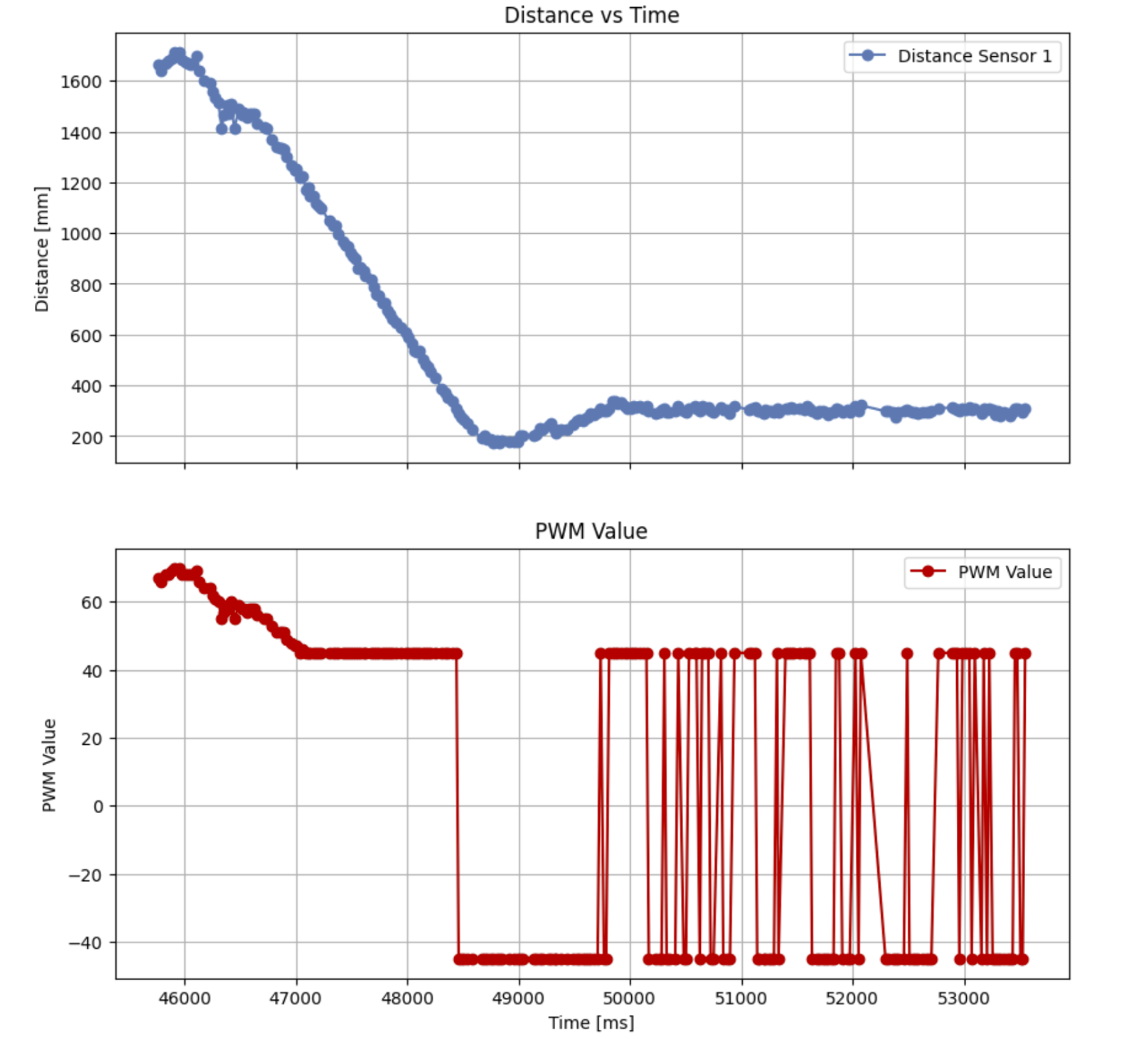
Figure 4: Plot of ToF and PWM vs time

Next, I added an Integral (I) term to eliminate steady-state error. The integral term accumulates the error over time and adjusts the PWM output accordingly:

This did not work well initially.

pid_dt= time_array[count]-time_array[count-1];
errP = (int)(distance - targetDist );
errI= (int) errI+ err*pid_dt;

pwm= (int) (kp*errP)+(ki*errI);

Figure 5: Initial Integral control implementation

PI is not looking good

Eventually I found and fixed my bug, but then got hit with some strong integrator windup.

Integrator Windup

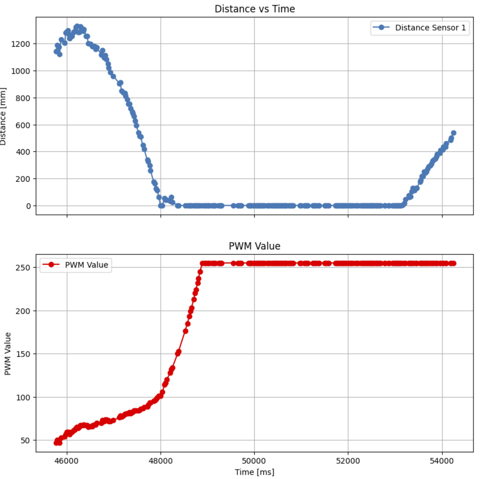
Figure 6: Plot of ToF and PWM vs time showcasing Integrator Windup

I set Ki = 0.01 to minimize steady-state error without significantly slowing down the system. However, even with this small value, windup grew rapidly. Thus I implemented a limit on the I term at +/- 150. (5000 level task).

if (errI > 150){
    errI=150;
}
else if (errI < 150){
    errI=-150;
}

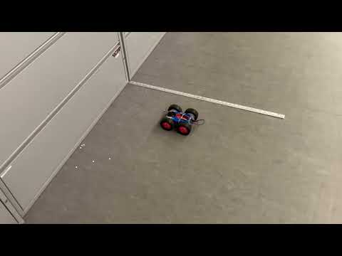
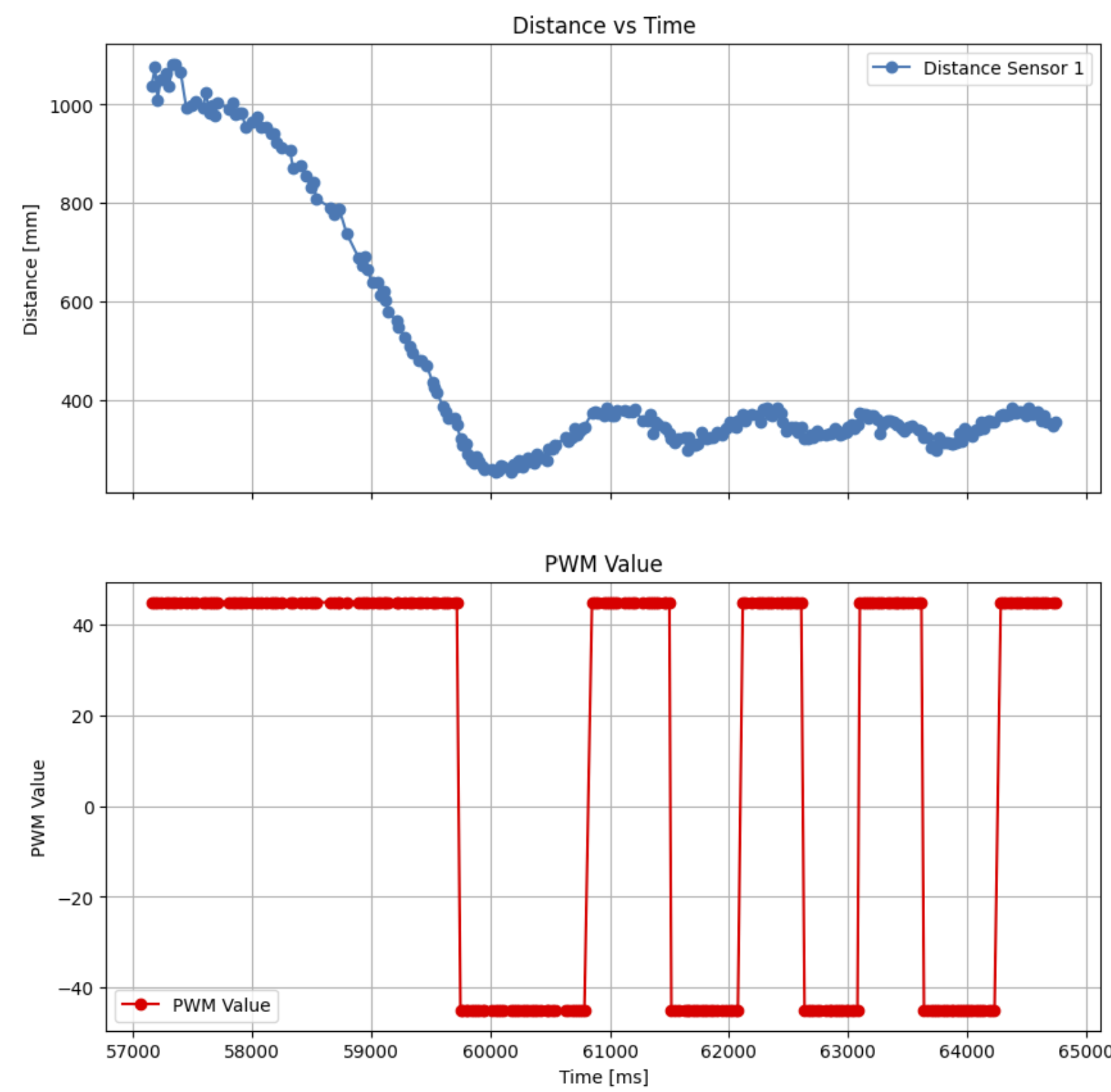
Figure 7: Plot of ToF and PWM vs time showcasing PI control

I’m not convinced that PI is actually helping for this use case as it seems to have amplified the oscillatory behavior. Depending on future lab goals, I may try to stick with well-tuned P-control. This needs further testing.

Range and Sampling Time

The ToF sensor was configured to operate in long-distance mode (up to 3.6 meters) and the control loop ran every ~20-40 ms, ensuring timely updates to the motor PWM values.

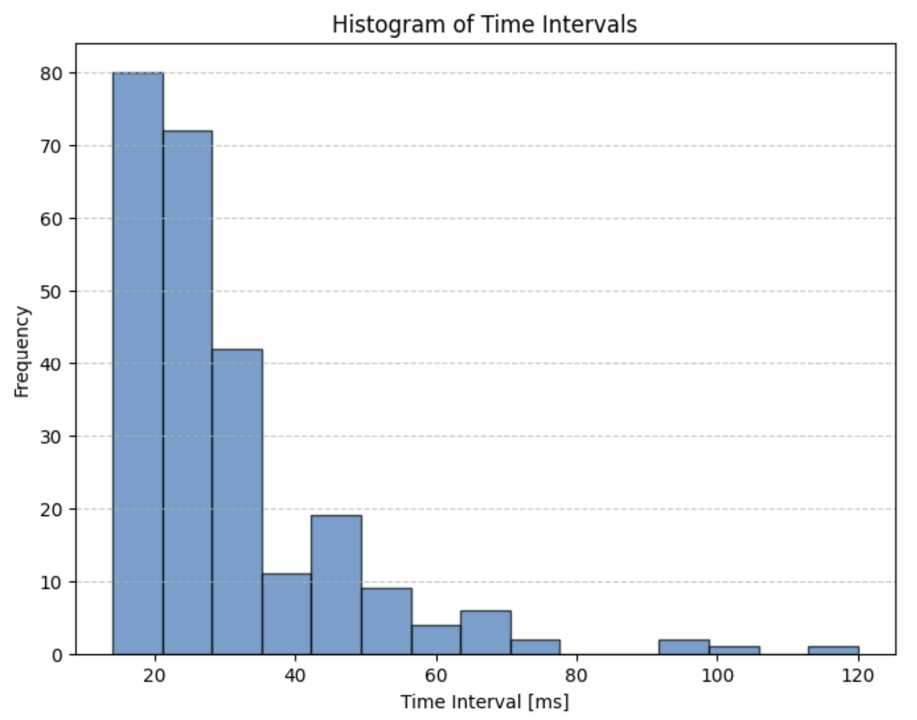
Figure 8: Histogram of Loop time intervals

The bulk of the loops took around 20-40 ms which is the minimum timing budget available for our ToF sensors, so I don’t think I can reasonably increase my speed beyond this limit since I’m currently waiting to begin each new loop until I have ToF data ready. However, this may be alleviated with linear extrapolation.

Linear Extrapolation

I implemented linear extrapolation to estimate the robot’s position when new ToF data was not available. This allowed the control loop to run much faster than the ToF sensor’s sampling rate:

 while (currMillisTOF - prevMillisTOF <= 10000) {
              distanceSensor1.startRanging();

              if (distanceSensor1.checkForDataReady()) {
                //normal pid

              }
              else if(count > 2){
                  count++;
                  float d1 = TOF_array[count-2]; 
                  float d2 = TOF_array[count-1];
                  float t1 = time_array[count-2]; 
                  float t2 = time_array[count-1];

                  float dxdt = (d2-d1)/(t2/1000-t1/1000);
                  float dx = dxdt * (millis()-t2);
                  float errP = (d2+dx) - targetDist;

                  // Serial.print("slope: ");
                  // Serial.print(dxdt);
                  // Serial.println(" | ");

                  //Proportional Control
                  int pwm = kp * errP;
                  time_array[count] = (int)millis();
                  TOF_array[count] = 0;
                  
                }
                
                //send pwm to motors
 }

Figure 9: Linear extrapolation implementation

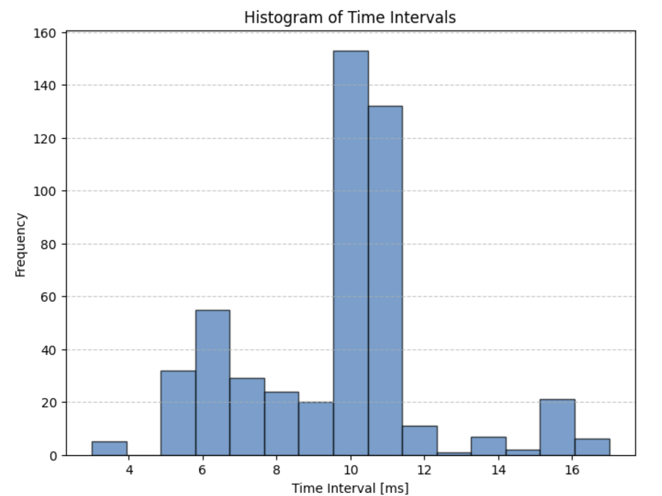
Figure 10: Histogram of Loop time intervals with Linear Extrapolation

The loop speed become way faster which is great. Unfortunately, the PID controller didn’t work as well as the previous versions so I’m not sure I’ll use this method for further testing.

Conclusion

This lab provided hands-on experience with PID control and highlighted the importance of tuning gains, managing sampling rates, and implementing safeguards like integrator windup protection. The robot successfully stopped at the target distance of 304 mm from the wall, demonstrating the effectiveness of the PI controller.