
Fast Robots - Lab 7: Kalman Filter
Prelab
The goal of this lab was to implement a Kalman Filter to execute the PID loop from Lab 5 faster and more efficiently. The Kalman Filter would help estimate the robot’s state (distance and velocity) by combining sensor measurements with predictions from our system model.
Kalman Filter Math
Based on some notes I took for another project, I already had a decent understanding of Kalman Filters.
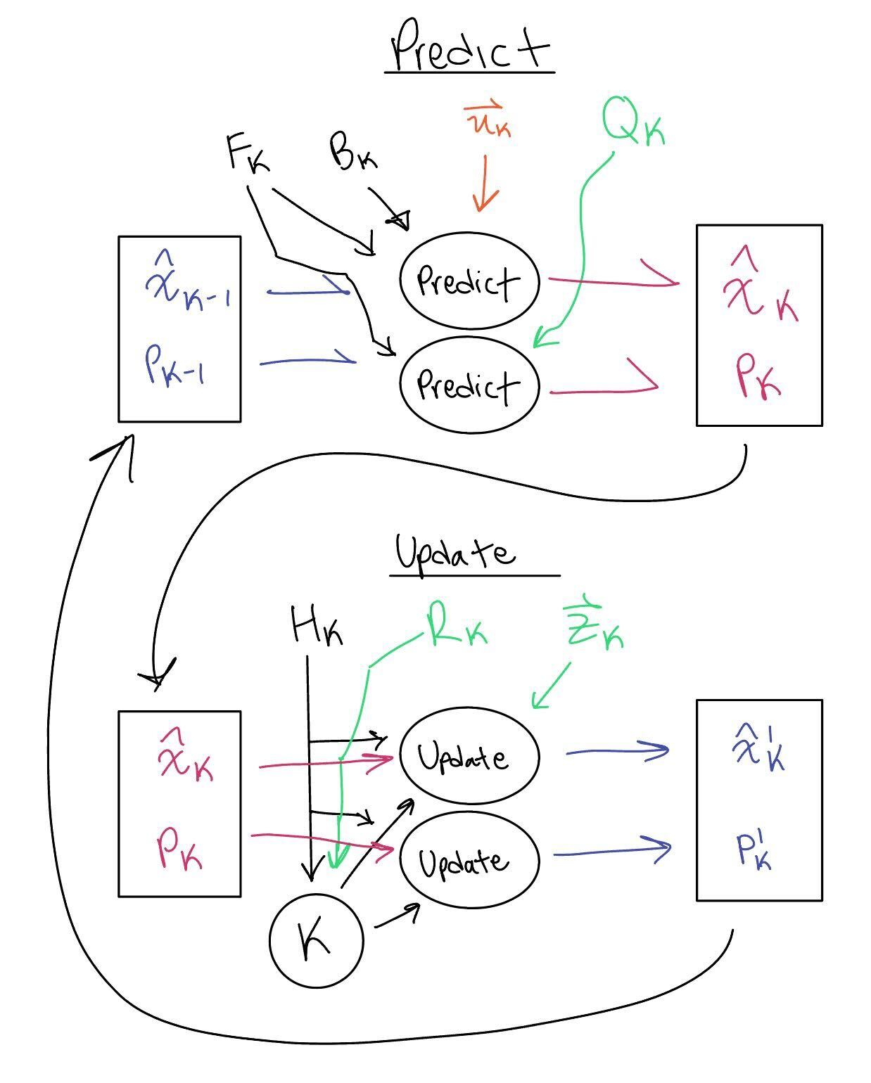
Figure 1: Kalman Filter Process Diagram
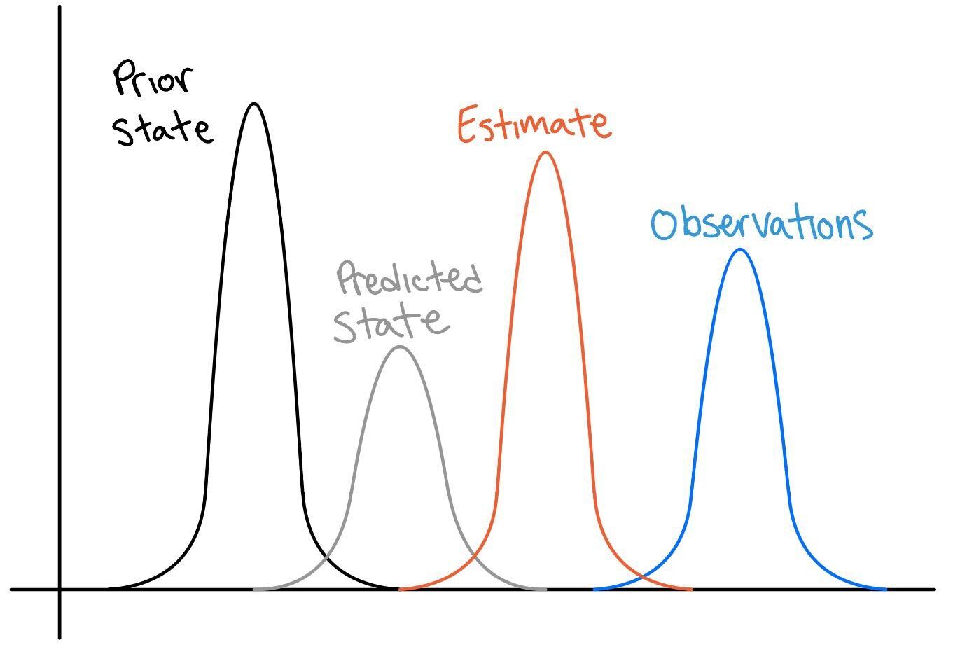
Figure 2: Kalman Filter Gaussian Overlay

Figure 3: Kalman Filter Math
Initially, I tried to implement a kalman filter utilizing my previous notes notation. However, I just ended up confusing myself by using a inchoerent mix of previous notation and notation from Fast Robots Lecture. Eventually, I decided to cut my losses and just maintain Fast Robots notation for consistency.
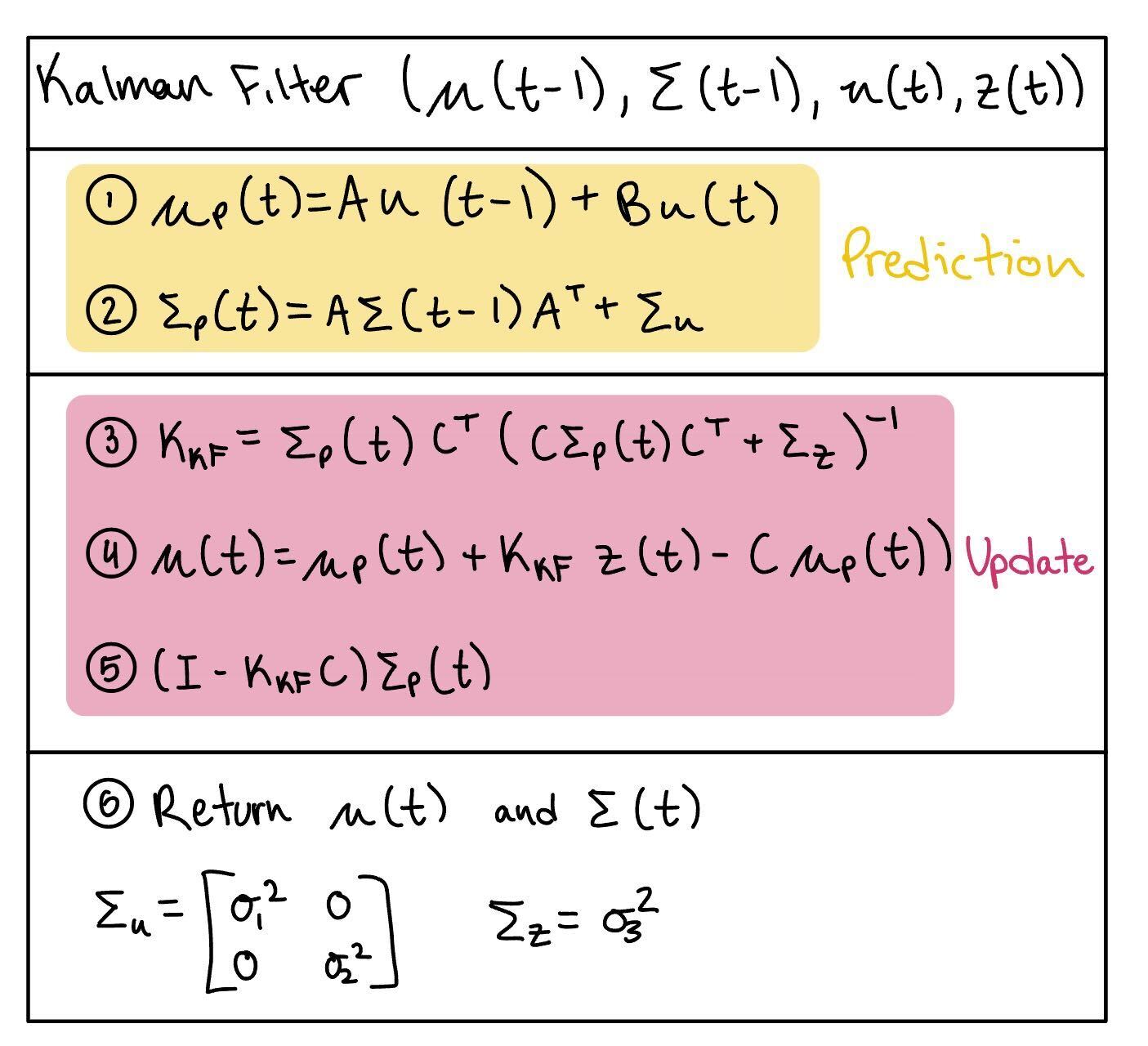
Figure 4: Kalman Filter Math with Fast Robots Notation
Estimating System Parameters
To implement the Kalman Filter, I first needed to estimate the drag (d) and momentum (m) parameters of my robot:
- Ran the robot at 175 PWM (~68% of max 255)
- Collected timestamped distance data from the ToF sensor
- Calculated velocity from the distance measurements
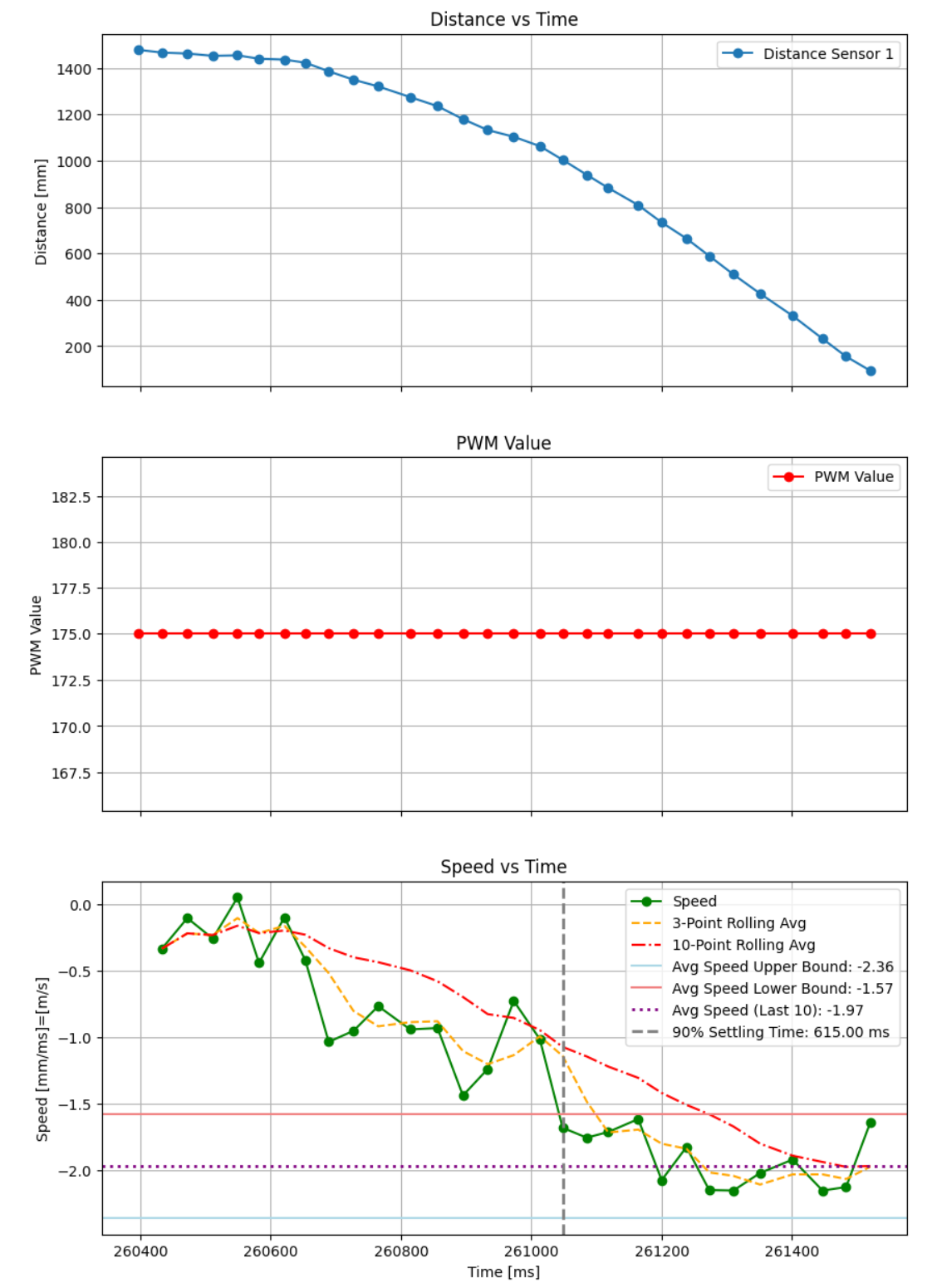
Figure 5: Kalman Filter Math with Fast Robots Notation
From the velocity vs time graph, I determined:
- Steady state velocity: 1.97 m/s
- 90% rise time: 615 ms
Kalman Filter Python Implementation
Using these values, I used python to calculate:
#d
uss= 175/255 # 175 pwm, max 255 pwm
xdot= 1.97 #m/s
d= uss/xdot
print("d: " ,d)
d: 0.34836269533193986
#m
t_r = 0.615
m = (-d*t_r)/np.log(0.1)
print ("m: ", m)
m: 0.0930445777144172
Next, I found covariance matricies using the equations from lecture slides:
A = np.array([[0,1],[0,-d/m]])
B = np.array([[0],[(1/m)]])
C = np.array([[-1,0]])

delta_t = avg_time # this comes from timing histogram (this value tends to be ~34-39 ms)
Ad = np.eye(2) + delta_t * A
Bd = delta_t * B

x = np.array([[-dist[0]],[0]])

sigma_1 = (10**2*1/delta_t)**0.5
sigma_2 = sigma_1
sigma_3 = 20
sig_u=np.array([[sigma_1**2,0],[0,sigma_2**2]])
sig_z=np.array([[sigma_3**2]])

print ("A: ", A)
print ("B: ", B)
print ("C: ", C)
print ("Ad: ", Ad)
print ("Bd: ", Bd)

print ("sig1: ", sigma_1)
print ("sig2: ", sigma_2)
print ("sig3: ", sigma_3)
print ("sig u: ", sig_u)
print ("sig z: ", sig_z)
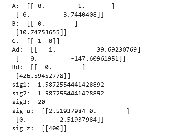
Figure 6: Computed KF matrix values
def kf(mu,sigma,u,y):

    mu_p = Ad.dot(mu) + Bd.dot(u)
    sigma_p = Ad.dot(sigma.dot(Ad.transpose())) + sig_u

    sigma_m = C.dot(sigma_p.dot(C.transpose())) + sig_z
    kkf_gain = sigma_p.dot(C.transpose().dot(np.linalg.inv(sigma_m)))

    y_m = y-C.dot(mu_p)
    mu = mu_p + kkf_gain.dot(y_m)
    sigma=(np.eye(2)-kkf_gain.dot(C)).dot(sigma_p)
    return mu,sigma

kfA = []
sig = np.array([[sigma_1,0],[0,sigma_1]])
for e, f in zip(pwms, dist):
    x,sig = kf(x,sig,[[e/80]],[[f]])
    kfA.append(-x[0,0])
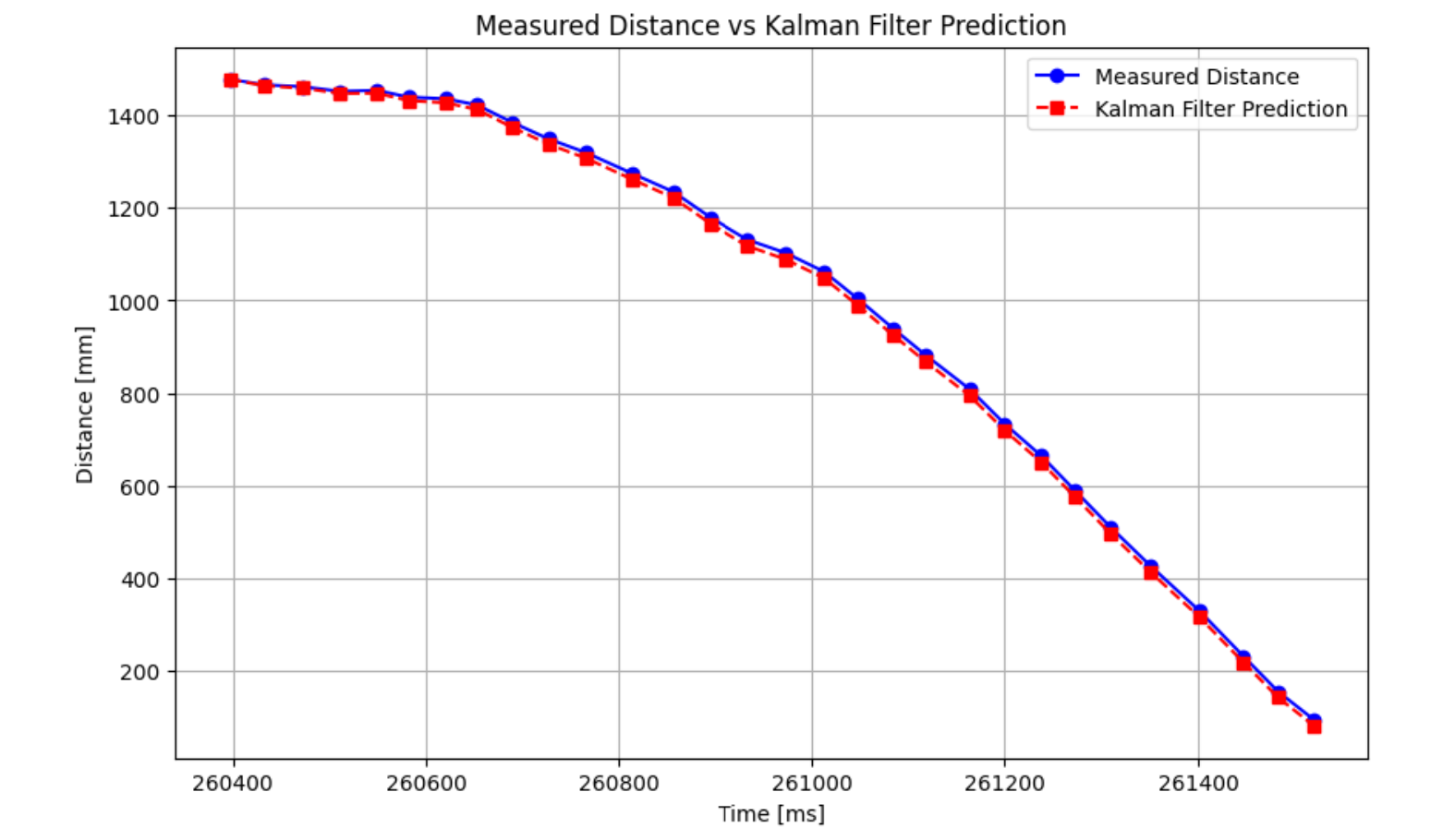
Figure 7: Kalman Filter Python implementation with initial data
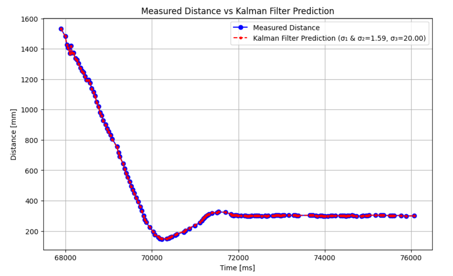
Figure 8: Kalman Filter Python implementation with PID data
The default sigma values using the heuristics and equations from lecture worked incredibly well, so I kept these values. I did try other combinations, but none were as good as the initial case. Thus, these are the values I will implement into my robot.
Kalman Filter Robot Implementation
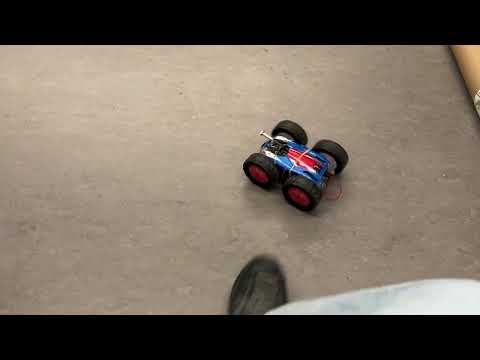
Figure 9: Kalman Filter Robot implementation video
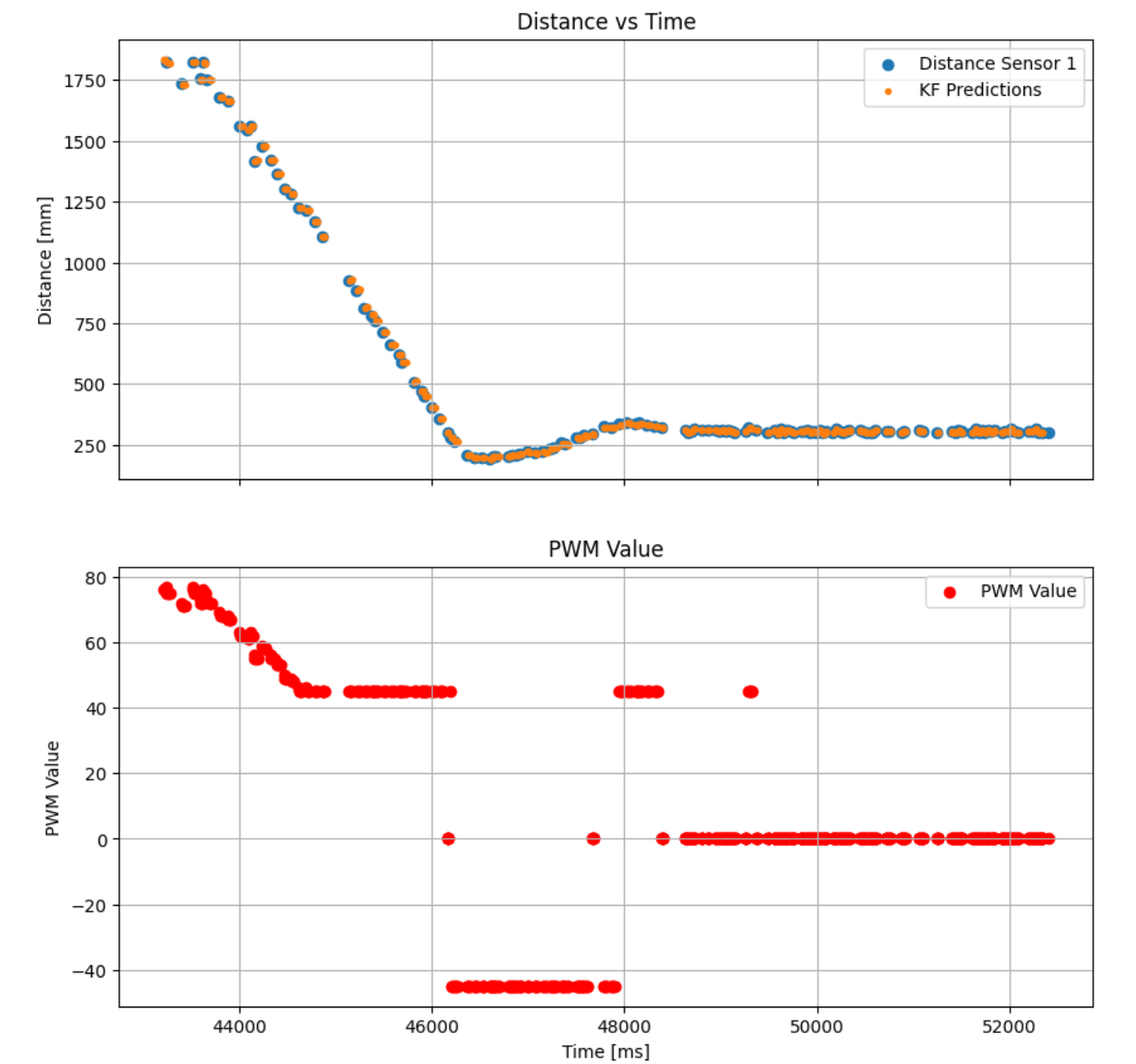
Figure 10: Kalman Filter Robot implementation with PID data
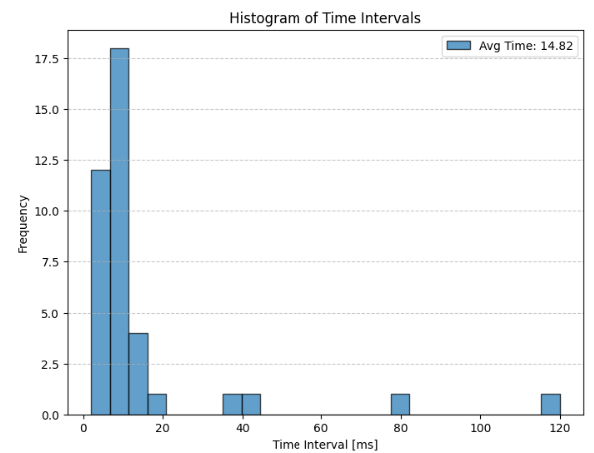
Figure 11: Kalman Filter Python implementation with PID data
During my first interations of KF implementation, I was estimating tens to hundreds of values between TOF sensor readings. This resulted in worse performance for my PID controller. To limit this, I set a cap of 5 estimated between TOF sensor readings. While fairly limited, this still resulted in a PID Loop time decrease of ~63% to an average of 14.82ms. This is quite a substantial improvement. I want to conduct further testing on the sweet spot for KF loop time during the stunt lab next week.
///////////////////////////////////////////////////////////////////////KF Vars+
float drag= 0.348362695;
float momentum= 0.348362695;
float kf;
float delta_t = 39.69/1000;

//A,B,C, I Matrices
Matrix<2, 2> A_kf = { 0, 1,
                      0, -drag / momentum };
Matrix<2, 1> B_kf = { 0,
                      1 / momentum };
Matrix<1, 2> C_kf = { -1, 0 };

Matrix<2, 2> I2 = { 1, 0,
                    0, 1 };
//Discretised A B
Matrix<2, 2> Ad = { 1, delta_t,
                    0, -147.609619 };
Matrix<2, 1> Bd = { 0,
                    426.59452778 };

//Initialise states
float sig1 = 1.587255;
float sig2 = sig1;
float sig3 = 20.0;

Matrix<2, 1> x_kf = { 1500.,
                      0 }; //int state
Matrix<2, 2> sig = { sig1, 0,
                     0, sig2 };

//Define noise covariance matrices
Matrix<2, 2> sig_u = { sig1 * sig1, 0,
                       0, sig2 *sig2 };
Matrix<1, 1> sig_z = { sig3 *sig3 };

// KF Function
void KF(float u, float y) {
  Matrix<1,1> u_matrix={u};
  Matrix<2,1> mu_p = Ad*x_kf + Bd*u_matrix;
  Matrix<2,2> sig_p = Ad*sig*(~Ad) + sig_u;
  Matrix<1,1> sig_m = C_kf*sig_p*(~C_kf) + sig_z;
  Invert(sig_m);
  Matrix<2,1> kf_gain = sig_p*(~C_kf)*(sig_m);
  Matrix<1,1> y_matrix = { y };
  Matrix<1,1> y_m = y_matrix - C_kf*mu_p;
  // Update
  x_kf = mu_p + kf_gain*y_m;
  sig = (I2 - kf_gain*C_kf)*sig_p;
}

///////////////////////////////////////////////////////////////////////KF Vars-
Figure 12: Kalman Filter Variables and helper function
    case PID_BEGIN:
      {

        while (currMillisTOF - prevMillisTOF <= 10000) {

          distanceSensor1.startRanging();
          if (distanceSensor1.checkForDataReady()) {
            time_array[count] = (int)millis();

            //Serial.print("tof: ");
            distance = distanceSensor1.getDistance();
            distanceSensor1.clearInterrupt();
            distanceSensor1.stopRanging();
            //Serial.print(distance);
            TOF_array[count] = distance*alpha+TOF_array[count-1]*(1-alpha);

            pid_dt = time_array[count] - time_array[count - 1];
            errP = (int)(distance - targetDist);
            errI = (int)errI + err * pid_dt / 1000;
            if (errI > 150) {
              errI = 150;
            } else if (errI < -150) {
              errI = -150;
            }
            //err= errP+errI;
            pwm= (int) (kp*errP)+(ki*errI);

            if (pwm > 0) {
              dir = 1;

            }

            else if (pwm < 0) {
              dir = -1;
            }
            pwm = abs(pwm);

            if (pwm < pwmMin) pwm = pwmMin;
            if (pwm > pwmMax) pwm = pwmMax;

            if ((errP<15) && (errP>-15)) pwm=0;
            driveStraight(dir, pwm);
            PWM_array[count] = (dir * pwm);
            currMillisTOF = millis();

            state=1;

            count++;
          }
          else if(state<5){
          time_array[count] = (int)millis();

          KF(pwm/175, -1*distance);
          distance= x_kf(0,0);
          kf_TOF_array[count]= distance;

          err = distance - targetDist;
          pwm = kp*err;
          if (pwm > 0) {
              dir = 1;

            }

            else if (pwm < 0) {
              dir = -1;
            }
            pwm = abs(pwm);

            if (pwm < pwmMin) pwm = pwmMin;
            if (pwm > pwmMax) pwm = pwmMax;

            if ((errP<10) && (errP>-10)) pwm=0;
            driveStraight(dir, pwm);
            PWM_array[count] = (dir * pwm);
            currMillisTOF = millis();
            delay(2);
            count++;
            state++;
          }

        }

        driveStraight(0, 0);  //stop driving

        Serial.println("send data");
        for (int i = 0; i < count; i++) {
          tx_estring_value.clear();
          tx_estring_value.append(time_array[i]);
          tx_estring_value.append(" | ");
          tx_estring_value.append(TOF_array[i]);
          tx_estring_value.append(" | ");
          tx_estring_value.append(PWM_array[i]);
          tx_estring_value.append(" | ");
          tx_estring_value.append(kf_TOF_array[i]);
          tx_characteristic_string.writeValue(tx_estring_value.c_str());
        }

        break;
      }
Figure 13: KF Robot Code